Math and science::Analysis

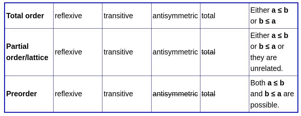
Order relations, visualized on graphs

Order relations can be visualized by how they can be represented by graph models. Partial orders, total orders, strict partial orders and strict total orders are introduced below property-by-property.

Starting from a set and a relation

The most general case begins with a set, \( A \), and a binary relation, \( R \), defined for \( A \). We will consider the binary relation to be defined as a function \( R : A \times A \rightarrow \{True, False\} \). For any elements \( a \) and \( b \) of \( A \), the value of the relation \( R \) is given by \( R(a, b) = a \le b \). Visualize this as a 2D table of boolean entries.

Directed graphs, enumerated

For two elements of \( A \), there are two possible values for \( R(a, b) \). As a graph, True can be encoded as the presence of a directed edge from \( a \) to \( b \).

There are four possible values of the pair of \( R(a, b) \) and \( R(b, a) \). If we include \( R(a, a) \) and \( R(b, b) \), we have 16 possible combinations. These combinations represent all possible directed graphs with two nodes where self-cycles are allowed.

Compressed representations

As we place restrictions on the possible combinations, more structure can be introduced into the graph model to compress the representation. The four types of order relations correspond to the following graph representations:

Partial order: Directed acyclic graph (with R(a, a) = True). Note that (I think) branching (in or out) is possible (e.g. R(a,b) = R(b,a) = False, while R(a,c) = R(b,c) = True).
Restricted partial order: There are many restrictions that can be introduced that introduce more structure, without becoming a total order. For example, a semi-lattice is a partial order with the rule that any two nodes must have common 'parent'. A semi-lattice is a slight generalization of a tree. In a semi-lattice, if direction of paths are ignored, then all nodes are connected.

Total order

The graph from a partial order with a significant restriction: there is only a single path, and it contains all nodes.

Strict partial order

Directed acyclic graph, (with R(a, a) = False)

Strict total order

All rules from strict partial order and total order.

Partial order

Starting from the general case. We introduce the following:

Reflexivity: Reflexivity removes the need represent self-cycles, as R(a, a) is always true.

Transitivity

Transitivity almost reduces the need for the graph model to have any cycles. In each connected component, there can be a single cycle. A graph can use paths to represet all relations: all nodes on a directed path have the relation \( a \le b \) where \( b \) is downstream of \( a \). Nodes within different connected components represent all elements \( n \) and \( m \) for which both \( R(n, m) \) and \( R(m, n) \) are false.

Antisymmetry, if \(R(a,b) \) and \( R(b,a) \) then \( a = b \)

Removes the need for any cycles. Our model becomes a true acyclic graph. There can be multiple connected components.

Total order

Carrying on from a partial order, we introduce one more restriction:

(What is the name for this?): for every \( a \) and \( b \) in \( A \), either \( a \le b \) or \( b \le a \).

This extra rule means that all elements of the set exist in a single connected component describing the relation.

Strict partial order

Strict partial order begins like partial order, but removes self-cycles in a different way, such that we don't later need antisymmetry in order to prevent cycles.

Irreflexivity: irreflexivity ( \( a \nless a \) for every \( a \) in \( A \)) removes the need for any loops, including self-loops. If \( a \) were in a loop, we would have \( a < a \), which this rule prohibits.
Transitivity: transitivity just like with the partial order case, transitivity allows paths to represent all values of the relation.

Strict total order

Like with the case of total order, we force all elements of the set to be part of the same connected component by introducing the restriction:

trichotomy: \( a < b \), \( a=b \), or \( a > b \) for every \( a \) and \( b \) in \( A \).

Pre-order

It's worth touching on pre-orders and where they fit in. A pre-order has even less restrictions than a partial order, and thus, the concept is more general.Specifically, we remove anti-symmetry.

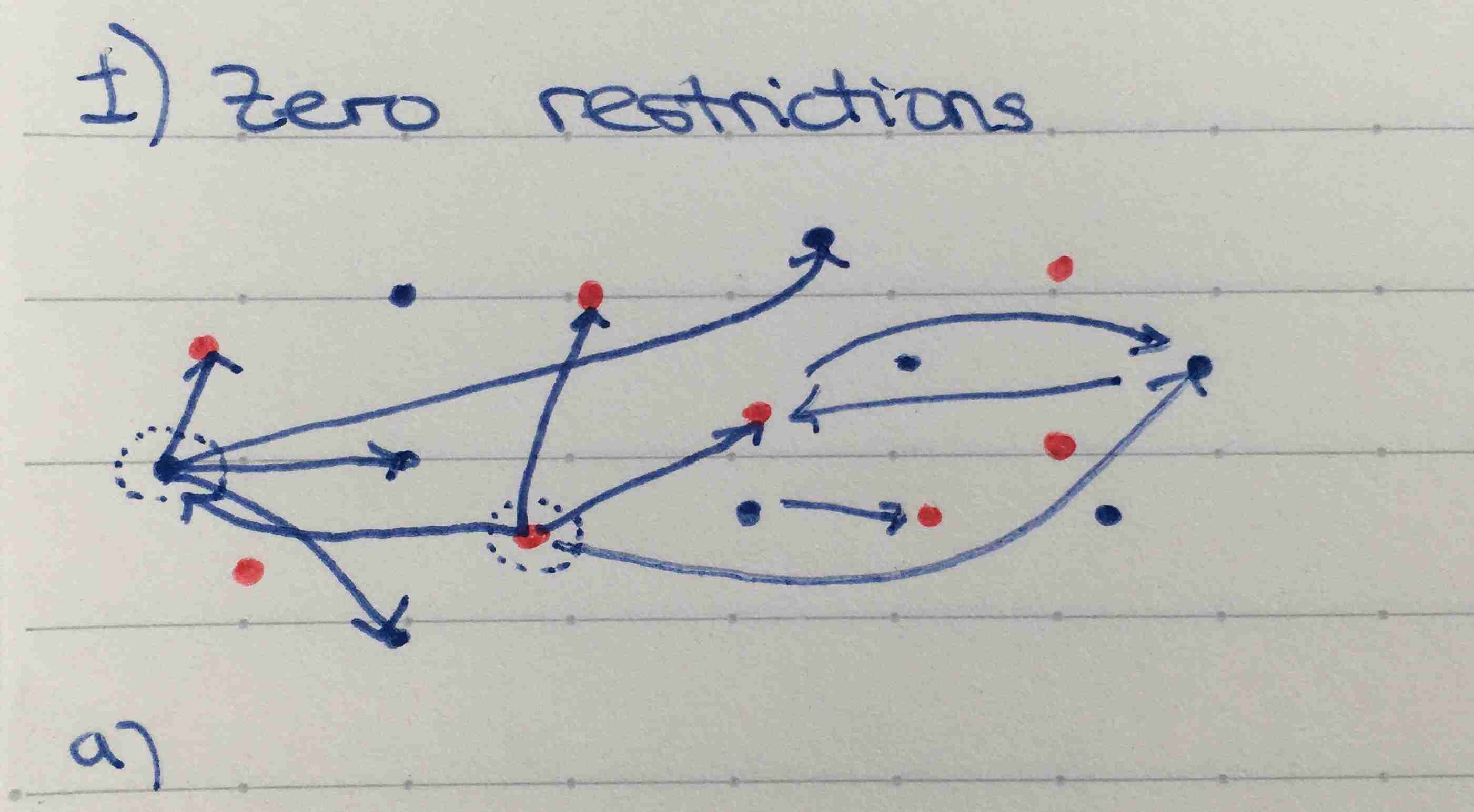
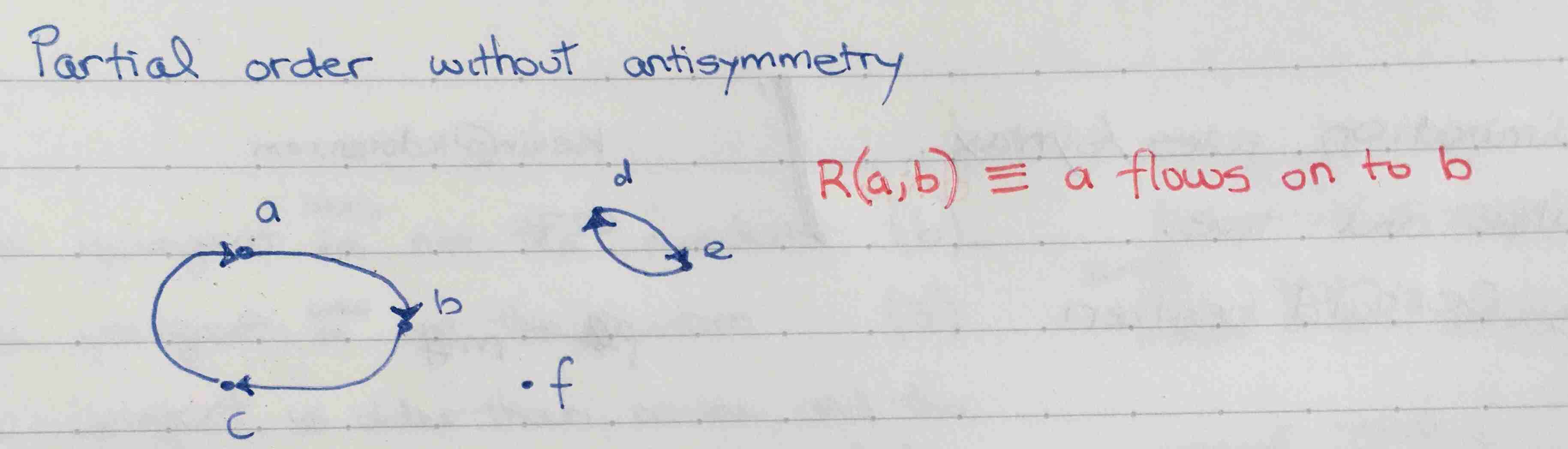
Some visuals:

Zero restrictions:

Transitivity almost removes all cycles:

Example of cycles that are permitted when there is no antisymmetry rule:

Relationship between partial and total order

The following two theorems reveal the close relationship between the two orders.

Theorem

Suppose ≤ is a partial order on a domain A. Define a<b to mean that a≤b and a≠b. Then < is a strict partial order. Moreover, if ≤ is total, so is <.

Theorem

Suppose < is a strict partial order on a domain A. Define a≤b to mean a<b or a=b. Then ≤ is a partial order. Moreover, if < is total, so is ≤.