
Multivariate Gaussian distribution
This card derives the general multivariate normal distribution from the standard multivariate normal distribution.
Standard multivariate Gaussian/normal distribution
Let \( (\Omega, \mathrm{F}, \mathbb{P}) \) be a probability space. Let \( X : \Omega \to \mathbb{R}^K \) be a continuous random vector. \( X \) is said to have a standard multivariate normal distribution iff its joint probability density function is:
As a vector of random variables
\( X \) can be considered to be a vector of independent random variables, each having a standard normal distribution. The proof of this formulation on the reverse side.
General multivariate
The general multivariate normal distribution is best understood as being the distribution that results from applying a linear transformation to a random variable having a multivariate standard normal distribution.
General multivariate normal distribution
Let \( (\Omega, \mathrm{F}, \mathbb{P}) \) be a probability space, and let \( Z : \Omega \to \mathrm{R}^K \) be a random vector with a multivariate standard normal distribution. Then let \( X = \mu + \Sigma Z \) be another random vector. \( X \) has a distribution \( f_X : \mathbb{R}^K \to \mathbb{R} \) which is a transformed version of \( Z \)'s distribution, \( f_Z : \mathbb{R}^K \to \mathbb{R} \):
Standard multivariate normal as a vector of independent random variables. Proof.
Proof that the above probability density function represents \( K \) independent standard normal random variables. For clarity, only the case when \( K = 3 \) will be highlighted:&= \frac{1}{ (2\pi)^{\frac{1}{2}} } \frac{1}{(2\pi)^{\frac{1}{2}}} \frac{1}{(2\pi)^{\frac{1}{2}}} e^{-\frac{z^Tz}{2}} \\
&= \frac{1}{(2\pi)^{\frac{1}{2}}} \frac{1}{(2\pi)^{\frac{1}{2}}} \frac{1}{(2\pi)^{\frac{1}{2}}} e^{-\frac{z_1^2 + z_2^2 + z_3^3}{2}} \\
&= \frac{1}{\sqrt{2\pi}} \frac{1}{\sqrt{2\pi}} \frac{1}{\sqrt{2\pi}} e^{-\frac{z_1^2}{2}} e^{-\frac{z_2^2}{2}} e^{-\frac{z_3^2}{2}} \\
&= \frac{1}{\sqrt{2\pi}} e^{-\frac{z_1^2}{2}} \frac{1}{\sqrt{2\pi}} e^{-\frac{z_2^2}{2}} \frac{1}{\sqrt{2\pi}} e^{-\frac{z_3^2}{2}} \\&= f(z_1) f(z_2) f(z_3) \end{aligned}\]
Thus, the propability distribution for \( Z \) represents 3 independent random variables having a individual distribution of \( \frac{1}{\sqrt{2\pi}}e^{-\frac{z_i^2}{2}} \) which is the standard normal distribution for a single random variable.
Elementwise conceptualization
The quantity \( [X - \mu] \Sigma^{-1} [X-\mu] \) can be thought of as a component wise operation, sum(\( \frac{[X - \mu ]^2}{\sigma^2} \)), where \( \sigma \) is the column vector of standard deviations. Another alternative is to imagine the component wise methods that would be called in a linear algebra/DL library: accumulate(mult(invert(pow(\( \sigma \), 2)), pow(\( X - \mu \), 2))).
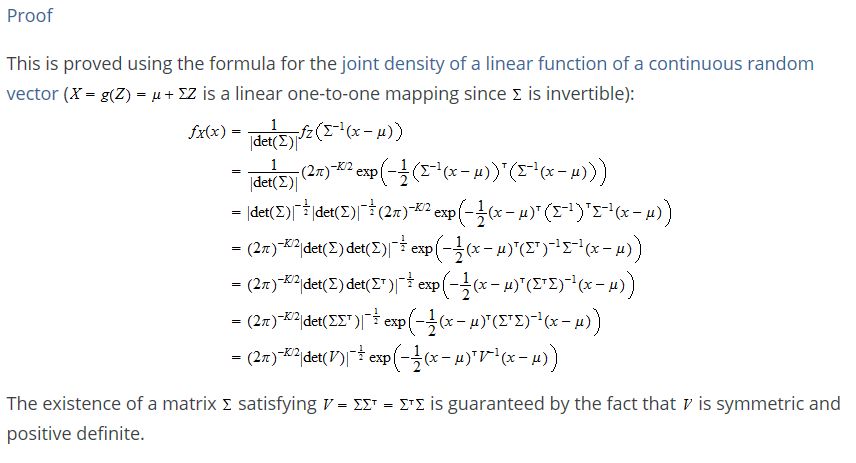
\(V = \Sigma^{\mathsf{T}} \Sigma \) form. Proof.
The Statlect formulation simplifies the expression. Copy-pasted here:
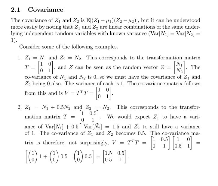
Dispelling the mystery of the co-variance matrix
Here is a screenshot of some notes on the perspective of a multivariate Gaussian random variable being a composition of two standard normal variables. It tries to dispell some of the mystery about why the co-variance matrix comes up the way it does.

Example
.PNG)