Covariance matrix and estimation
Yet another card on covariance and covariance matrices.
There is a good card on covariance, which I recap here:
Covariance is a real that gives some sense of how much two variables are linearly related to each other, as well as the scale of these variables. Covariance is a function of a probability space and two random variables. Let \( (\Omega, \mathrm{F}, \mathbb{P}) \) be a discrete probability space let \( X: \Omega \to S_x \) and \( Y : \Omega \to S_y \), be two random variables, where \( S_x\) and \( S_y \) are finite subsets of \( \mathbb{R} \). Then the covariance of \( X \) and \( Y \) is:
If instead the probability space is continuous, we can still define covariance, we will just employ an integral for the expectation.
The essense of this definition
This definition describes covariance as a function of two random variables, \( X : \Omega \to \mathbb{R} \) and \( Y : \Omega \to \mathbb{R} \). Optionally, this can be expressed as a function of a 2D random variable \( \vb{X} : \Omega \to \mathbb{R}^2 \).
Another perspective is that covariance is the expectation of the random variable \( Z : \Omega \to \mathbb{R} \), \( Z = (X-\mathrm{E}[X])(Y - \mathrm{E}[Y]) \).
Covariance matrix
Just a small step from the previous discussion brings us to the matrix product:
The elements of these vectors and matrices are functions/random variables. If we take the elementwise expectation of the matrix above, we arrive at the covariance matrix:
This is a matrix containing 4 real numbers; each expectations over random variables defined on the sample space.
If we make the synatic change to use a multivariate random variable, where \( X \) and \(Y \) are now the vector components \(\vb{x}_1\) and \( \vb{x}_2 \), we arrive at the notation:
where the expectation of a matrix is defined to be an elementwise application of the 1D expectation operation. It is worth mentioning that we are invoking the definitions of random vectors and matricies, and the expectation of these. These are indeed commonly defined notions, for example, Statlet defines random vectors and random matrices, and also covers them when defining expectation.
Essence of covariance matrix
The covariance matrix is an expectation applied to a matrix of random variables.
If we zoom, we can view the covariance matrix as being the output of an operation which takes in a random vector (function) on a probability space, \(( \Omega, \mathrm{F}, \mathbb{P}) \), and producing a matrix of reals. The operation has an intermediate output taking the form of a random matrix (random vector → random matrix → element-wise expectation). In this sense, the operation is comparable to the expecation or variance operation, it just has a higher dimensional output.
If we were to determine the values (reals) of the covariance matrix,
we would need to know \( \mathbb{P} \) and the random vector involved.
Data covariance matrix
When one has some data, it is often said that one can compute the covariance matrix of the data.
There is a little bit of ambiguity as to the exact calculation to run ( \( \frac{1}{n} \) or \( \frac{1}{n-1} \) factor?), and a related ambiguity as to what the matrix represents (an unbiased estimator of the covariance matrix, or a MLE of some model parameter?).
The 1-dimensional data case (which doesn't have any concept of covariance) can motivate the 2+-dimensional case.
1-dimension case
Given some 1D data, we can consider the data to be samples of a random variable \( X : \Omega \to \mathbb{R} \). The best way to conceptualize \( n \) samples is that it is \( n \) draw from sample space \( \Omega \), or 1 draw from \( \Omega^n \), and then the random variable \( X : \Omega \to \mathbb{R} \) is applied to each draw, so that we get \( n \) possibly different values \( X_1, X_2, ..., X_n \).
If the samples are reals, then the random variable \( Z : \mathbb{R}^n \to \mathbb{R} \) defined by \( Z = \frac{1}{n} \sum_{i=1}^{n} X_i \), which redistributes the n-dimensional distribution back to 1D, has an expected value \( \mathrm{E}[Z] \) which is equal to \( \mathrm{E}[X] \), where \( X : \Omega \to \mathbb{R} \), the 1D random variable. In this way, \( Z \) is a non-biased estimator for \( \mathrm{E}[X] \). In this sense, we are estimating the value of the expectation operator applied to the random variable \( X \); we don't need to know anything about the nature of the distribution created by \( X \).
Similarly, the random variable \( W = \frac{1}{n - 1}(X_1 - \mathrm{E}[X])(X_2 - \mathrm{E}[X])...(X_n - \mathrm{E}[X]) \) is an unbiased estimate for the expectation operator applied to the random variable \( (X - \mathrm{E}[X])^2 \) (i.e. the variance operator applied to \( X \)).
The case below is simply the same idea applied to data which itself has more than 1 dimension.
d-dimension case
If each sample is not 1 but \( d \) dimensions, then we must consider a random vector \( X : \Omega \to \mathbb{R}^d \). \( n \) samples of this can be represented by a vector of random vectors: \( n \)-dimensional vector of \( d \)-dimensional vector valued random variables. Like above, we may consider composing new random vectors which project back to \( \mathbb{R} \) and which have an expectation equal to something interesting. For example, we can create \( d \) different random variables which average a single component of the data across all samples: \( Z_j : \mathbb{R}^n \times \mathbb{R}^d \to \mathbb{R}\) defined by \( Z_j(X) = \sum_{i=1}^{n} W_{ji} \), if we assume that \( W \) is a matrix that collects together the random vectors \( X_1, ... X_n \) as columns (data expands horizontally). These random variables have an expectation equal to the mean of the marginalized \( j \) component of the random vector \( X \).
We can also try create estimators for the variance of each component of \( X \) and for the covariance between different components. What is nice is that the factor \( \frac{1}{n-1} \) that we would expect to appear in the estimator of a single 1D component–this factor is also required for estimating covariance between components, for conceptually the same reason.
Matrix calculations
If we have a finite list of \( n \) \( d \)-dimensional data points, we can package them together into a matrix \( \vb{X} \), with each of the \( n \) data points being a \( d \)-element column of the matrix.
Note on matrix layout
The above data-as-column layout is useful if we wish to consider \( \vb{x'} = \vb{Mx} \) as a transformation matrix \( \vb{M} \) being applied to the data vectors in \( \vb{x} \). If instead we have rows of \( \vb{x} \) representing data points, then \( \vb{xM} \to \vb{x'} \) is a better representation of the transformation operation.
Covariance estimator
From the data we can calculate a sample covariance matrix \( \vb{S} \), defined as:
Where \( \overline{\vb{x}} \) is the data mean:
Sometimes, the data mean is zero, \( \overline{\vb{x}} = 0 \). An we have:
MLE for normal random variable
If you know that the random variable is a multivariate normal random variable, and you wish to estimate the model parameter \( \Sigma \), then it turns out that the MLE for this is:
- a non-biased estimation for the multidimensional random variable's covariance matrix (for any arbitrary random variable)
- the most likely parameterization for a multivariate normal variable which generates the observed samples
Important distinction: random vector vs. vector of random variables
- Random vector
- With a sample space \( \Omega = [0, 1] \), the elements \( X_i \) of a random vector \( X : \Omega \to \mathbb{R}^d \) are each a function \( X_i : \Omega \to \mathbb{R} \) from the sample space. This random vector can be used to represent \( d \)-dimensional data.
- Vector of random variables
- When we wish to represent \( n \) samples, we are instead dealing with a \( n \)-dimensional sample space \( \Omega = [0, 1]^n \), and a vector of random variables \( [X_1, X_2, X_3,..] \) where each random variable \( X_i : \Omega \to \mathbb{R} \) maps from one of the components of \( \Omega \). These random variables in effect come from different sample spaces. If the samples themselves are \( d \)-dimensional, then the \( n \) samples takes the form of a matrix, or a vector of vector valued random variables.
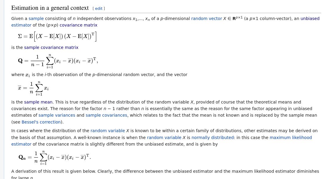
More on estimator vs multivariate MLE
The wikipedia page has a nice section: