
Monte Carlo Methods
The this card describes Monte Carlo methods in the words of David MacKay. A lot of this card's content is drawn from Chapter 29 of MacKay's book.
Monte Carlo methods. Definition.
Monte Carlo methods is a term for something that utilizes a random number generator to solve one or both of the following problems.
- Generate a sequence of samples \( (\vb{x}_i)_{i=1}^{R} \) from a given probability distribution, \( \mathbb{P}(\vb{x}) \).
- Estimate expectations of functions under this probability distribution.
For example, for some function \( \phi \), we want to know:
\[ \int {\dd}^N \vb{x} \; \mathbb{P}(\vb{x}) \phi(\vb{x}) \]
The notation used above does a lot of heavy lifting. "\( \mathbb{P}(\vb{x}) \)" suggests a set \( L \subset \mathbb{R}^N \) is the co-domain of an implied random variable \( Y : ? \to L \). \( L \) is also the domain of the function \( \mathbb{P} \) which must have a signature of the form \( \mathbb{P} : L \to \mathbb{R} \). The function \( \phi \) seems to have a signature \( \phi : L \to \mathbb{R} \). It is composed with \( Y \) like \( \phi \circ Y \) and thus, \( \phi \) is a random variable. The composition implies that the domain of \( \phi \) is \( L \). The integration formula further implies either that the co-domain of \( \phi \) must be \( \mathbb{R} \) (alternatively, the integration is syntax is allowing for the interpretation of a vector valued integration which seems a stretch).
The reverse side describes Lake plankton analogy to the above problems. Can you remember the details? The reverse side also rewords the above description in the language of probability distributions.
Lake plankton analogy
Imagine the task of trying to determine the average plankton concentration of a lake. You are provided with a boat, GPS and a plankton sensor attached to a plumbline. To make this analogy work, we assert that the plankton concentration is vertically uniform. These tools allow you to sample a single 1cm3 volume of the lake and determine its plankton concentration.
The depth of the lake at position \( \vb{x} = (x, y) \) is given by \( \mathbb{P}^*(\vb{x}) \). The plankton concentration \( \phi(\vb{x}) \) is also function of the position on the lake. The average plankton concentration is then:
Outside of the analogy, the quantity \( \frac{\mathbb{P}*}{Z} = \mathbb{P} \) is the true, normalized probability.
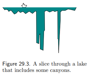
The fact that the depth of the lake is unknown makes it very difficult to calculate \( Z \), and thus, it is very difficult to know how significant a single sample is to the overall calculation. MacKay brought up the example of a lake with narrow deep canyons. This canyon has a large effect on the average concentration; however, it is easy to miss sampling from it altogether. To do a good job of sampling, we must somehow discover the canyons and discover their depth and width relative to the rest of the lake.
Maybe a better analogy is the task of measuring the amount of gold in a gold deposit. Vertical core samples can be taken by pulling out a thin cylindrical sample all the way down to some hard impenetrable rock. The depth of the impenetrable rock is unknown. Trying to infer the total gold deposit from a few samples is a difficult problem that corresponds to the roughly to the second problem (although, it is a bit different).
Monte Carlo methods. More Formal.
An attempt to formulate the ideas using the language of probability spaces might describe Monte Carlo methods as follows.
The two problems that Monte Carlo methods are to solve
Let \( (\Omega, \mathrm{F}, \mathbb{P}) \) be a probability space. Let \( X : \Omega \to \mathbb{R} \) be a random variable. \( \mathbb{P} \) and \( X \) determine the probability distribution \( \mathrm{F}_X : \mathbb{R} \to \mathbb{R} \) of \( X \). In this context, the two problems to be solved are:- Generate a sequence of samples \( (\vb{x}_i)_{i=1}^{R} \) (where \( \vb{x}_i \in \mathbb{R}^d \)) such that the samples seem to be drawn from \( \mathrm{F}_X \).
- To estimate \( \mathrm{E}[X] \) and also estimate \( \mathrm{E}[Y] \) for some random variable \( Y = g(X) \) formed with a function \( g : \mathbb{R}^d \to \mathbb{R}^{d_2} \).
The description of the first problem is discussed in more detail below in Generating a random sequence.
To solve these problems we are allowed to assume the existence of a sequence \( (r_i)_{i=0}^{\infty} \) which represents our access to a random number generator. (TODO: what is the formulation of this sequence in terms of probability spaces and random variables?). A solution to the two problems that utilize this sequence constitutes a Monte Carlo method. What defines a solution is another facet of the situation.
Generating a random sequence
Only in attempting to write the first problem in terms of probability spaces have I realized that it's not obvious how to transition from the ideas of probability spaces to the ideas of generating samples. A lot is glossed over in the words seems to be drawn from. Maybe a better description is to say something like, as \( R \to \infty \), the random variable \( Z : \mathbb{N} \cap [1, R] \to \mathbb{R} \) on the sample space \( \Omega = \mathbb{N} \cap [1, R], \mathrm{F}, \mathbb{P}) \) (with \( \mathbb{P}(\{i\}) = \frac{1}{R} \) and \( \mathrm{F} \) being every subset of \( \Omega \)) has a probability distribution \( \mathrm{F}_X \) that approaches \( \mathrm{F}_X \). This raises more questions about discrete vs. continuous, so I think I'll stop with this thread.