Importance sampling and rejection sampling

Rejection sampling is useful for generating samples that are distributed according to a difficult-to-sample-from distribution.

Importance sampling is useful for evaluating a function (such as expectation) of a random variable with a difficult-to-sample-from distribution.

Common setup

Let \( P(x) \) be a distribution which we can evaluate an unnormalized version of easily at a point to obtain \( P^*(x) \). \( P(x) = \frac{P^*(x)}{Z} \) where \( Z = \int P^*(x) \dd{x} \). 

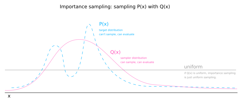
Importance sampling

Propose we have a function \( \phi(x) \) for which we wish to evaluate an expectation. We may proceed with uniform sampling by taking \( R \) samples of a uniform distribution over the domain, \( x_1, x_2, ... x_R \) and calculating an estimate:

Importance sampling alters this calculation by sampling domain values from a distribution other than the uniform distribution. Let \( Q(x) \) be the sampler distribution. We will sample \( R \) samples from the sampler distribution and estimate the expectation of \( \phi \) like so:

The sampler distribution has two effects:

1. It focuses where in the domain \( x \) is sampled.
2. It causes the estimation of the normalizing \( Z_P\) constant to be skewed by oversampling some values and undersampling others.

The first effect is beneficial and the second is not. The second effect can be conceptualised  as \( Q(x) \) stretching the domain in some places and shirking it in others. The size of the domain is important as a measure by which we are weighting the \( P^*(x) \) that we are collecting. To counteract the undesired effect of \( Q(x) \), we simply multiply \( P^*(x) \) by \( \frac{1}{Q(x)} \). Any part of the domain that is stretch by \( Q(x) \) shrinks the weight given to a \( P^*(x) \) sample by multiplying by the reciprocal amount.

The fact that we multiply \( \phi(x) \) by \( P^*(x) \) fully accounts for the weighting for \( \phi \). The \( \frac{1}{Q(x_0)} \) factor is simply to undo the fact that we are going to be sampling point \(x_0 \) excessively according to the value \( Q(x_0) \). 

Rejection sampling

Rejection sampling is more true to it's "sampling" label, as it works to generate samples for a target distribution. The proceedure is very similar to importance sampling. It differs by sampling a second random variable \( u \) that is uniformmly distributed on the interval \( [0, \; cQ^*(x) \,] \). Then, if \( u \leq P^*(x) \), the sample \( x \) is kept, else it is rejected.

Inhomogeneous Poisson sampling: thinning

Rejection sampling applied to sampling an inhomogeneous Poisson distribution defined by a variable hazard function is called "thinning" (introduced by Lewis and Shedler (1979)).