
Experiment 1.6.1
A green-blue version of 1.5, carried out for the purposes of comparison.A green-blue dataset similar to the orange-brown dataset will be programatically created and tested just like in 1.5.
import os
import pickle
import time
import copy
import pathlib
import itertools
from collections import namedtuple
from enum import Enum
from typing import *
import IPython
import cv2
import numpy as np
import torch.optim
import torch.hub
import torchvision as tv
import torchvision.datasets
import torchvision.models
import torchvision.transforms
import matplotlib.pyplot as plt
import matplotlib as mpl
import pandas as pd
import colorsys
from icecream import ic
import nncolor as nc
import nncolor.data
presentation_mode = True
if presentation_mode:
    import warnings
    plt.style.use('science')
    warnings.filterwarnings('ignore')
    mpl.rcParams.update({'font.size': 30})
    mpl.rcParams.update({'axes.labelsize': 30})
    mpl.rcParams.update({'text.usetex': True})
import IPython
def imshow(img):
    """Show image.

    Image is a HWC numpy array with values in the range 0-1."""
    img = img*255
    img = cv2.cvtColor(img, cv2.COLOR_RGB2BGR)
    # cv2 imencode takes images in HWC dimension order.
    _,ret = cv2.imencode('.jpg', img)
    i = IPython.display.Image(data=ret)
    IPython.display.display(i)
1. Notebook constants
Variables used as constants throughout the notebook.
EXPERIMENT = '1_6_1'
# Choose CPU or GPU.
device = torch.device('cuda:1')
#device = "cpu"

# Choose small or large (standard) model variant
model_name = 'resnet50'
def model_fctn():
    if model_name == 'resnet18':
        return tv.models.resnet18(pretrained=True)
    elif model_name == 'resnet50':
        return tv.models.resnet50(pretrained=True)
resnet_model = model_fctn()

IMG_SHAPE = (224, 224, 3)
GRID_SHAPE = (1, 1)
CENTER_ACTIVATION = 0 # position (1, 1) in grid of 1x1
NUM_CELLS = 1
cell_shape = nc.data.cell_shape(GRID_SHAPE, IMG_SHAPE)
assert np.array_equal(cell_shape, IMG_SHAPE[0:-1])
BATCH_SIZE = 64
NUM_EPOCHS = 20
NUM_FC_CHANNELS = 512 if model_name == 'resnet18' else 2048
SAVE_PATH_FMT = './resources/exp_' + EXPERIMENT + '/{model_name}_radius_{radius}_offset_{offset}_save'
ACC_SAVE_PATH = './resources/exp_' + EXPERIMENT + f'/{model_name}_accuracy.json'
2. Dataset
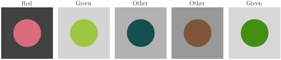
Here we try to create a similar dataset to the orange-brown dataset, but with two colors that can be distinguished with hue, rather than relative brightness. The class weights are kept the same, with the number of red classifications matching those of orange in the orange-brown data set. Similarly, green maps to brown, and neither to neither, which carries the same meaning in both datasets. The dataset is created programatically; however, the settings were experimentally tested to insure they would not create incorrect classifications.
# Variations by dot position, offset from center along south-east diagonal.
# 15 different offsets, from 0 to 112 inclusive.
# 112 / 8 = 14
offsets = list(range(0, 112+1, 8))
assert len(offsets) == 15
# Varations, by dot radius.
# 29 different offsets from 0 to 168 inclusive. 0 is replaced by 1 for the first radius.
# 168 / 6 = 28.
radii = [1,] + list(range(6, 168 + 1, 6))
assert len(radii) == 29
class RedGreenData:

    RED = 0
    GREEN = 1
    OTHER = 2

    def __init__(self, num_red, num_green, num_other):
        self._rng = np.random.default_rng(345)
        self.red = []
        self.green = []
        self.other = []
        self._populate(num_red, num_green, num_other)

    def _random_color_pair(self):
        gray_rgb = np.array([self._rng.random()]*3)
        circle_hsv = self._rng.random(size=3)
        return (circle_hsv, gray_rgb)

    def _populate(self, num_red, num_green, num_other):
        def fin():
            fin =  len(self.red) >= num_red and \
                   len(self.green) >= num_green and \
                   len(self.other) >= num_other
            return fin

        while not fin():
            c,bg = self._random_color_pair()
            if self.is_red(c):
                self.red.append((self.RED, colorsys.hsv_to_rgb(*c), bg))
            elif self.is_green(c):
                self.green.append((self.GREEN, colorsys.hsv_to_rgb(*c), bg))
            elif self.is_other(c):
                self.other.append((self.OTHER, colorsys.hsv_to_rgb(*c), bg))
            else:
                continue
        self.red = self.red[:num_red]
        self.green = self.green[:num_green]
        self.other = self.other[:num_other]
        self.data = np.concatenate([self.red, self.green, self.other])
        self._rng.shuffle(self.data)

    @staticmethod
    def is_red(hsv):
        hsv = hsv * [360.0, 100.0, 100.0]
        res = (hsv[0] >= 350 or hsv[0] <= 8) and (hsv[1] >= 50) and (hsv[2] >= 30)
        return res

    @staticmethod
    def is_green(hsv):
        hsv = hsv * [360.0, 100.0, 100.0]
        res = (70 <= hsv[0] <= 155) and (hsv[1] >= 50) and (hsv[2] >= 50)
        return res

    @staticmethod
    def is_other(hsv):
        hsv = hsv * [360.0, 100.0, 100.0]
        res = (18.0 <= hsv[0] <= 60.0 or 165.0 <= hsv[0] <= 340.0) and \
            (hsv[1] >= 50) and (hsv[2] >= 30)
        return res

orange_brown_data = pd.read_csv('./resources/experiment_1_1_combined_edited.csv')
num_orange, num_brown, num_other = orange_brown_data['ans'].value_counts()[[0, 1, 3]]
red_green_data = RedGreenData(num_orange, num_brown, num_other).data.tolist()
Below are some samples from the dataset.
def show_examples():
    fig = plt.figure(figsize=(17, 7))
    ds = nc.data.ColorDotDataset(red_green_data,
                                       grid_shape=GRID_SHAPE,
                                       dot_radius=60)
    # Offset was chosen to find five continuous samples that contained all classes.
    offset = 7
    cols = 5
    for i in range(cols):
        ax = fig.add_subplot(1, cols, i+1)
        ax.set_axis_off()
        ax.imshow(ds[i+offset]['image'])
        label_id = ds[i+offset]['label']
        if label_id == 0:
            label = 'Red'
        elif label_id == 1:
            label = 'Green'
        else:
            label = 'Other'
        ax.set_title(label, fontsize=22)
    fig.subplots_adjust(hspace=0.10, wspace=0.10)
    plt.savefig("./out/report/nn_dataset_rg.pdf", format="pdf", bbox_inches="tight")
    plt.show()
show_examples()
# Data augmentation and normalization
normalize_transform =  tv.transforms.Normalize([0.485, 0.456, 0.406], [0.229, 0.224, 0.225])
to_CHW_tensor_transform = tv.transforms.ToTensor()
data_transform = tv.transforms.Compose([to_CHW_tensor_transform, normalize_transform])

def datasplits_by_pos_and_radius():
    """Create the datasets."""
    color_data = nc.data.exp_1_1_combined_data
    # We are ignoring the very few data points labeled "both".
    color_data = color_data[color_data['ans'] != nc.data.LABEL_TO_COLOR_ID['both']]
    color_data = nc.data.deserialize(color_data)
    def train_test_val(offset, radius):
        train_ds, test_ds, val_ds = nc.data.train_test_val_split(color_data,
                                                                dot_radius=radius,
                                                                grid_shape=GRID_SHAPE,
                                                                dot_offset=(offset, offset))
        DataSplit = namedtuple('DataSplit', ['ds', 'loader', 'size'])
        splits = {
            'train': DataSplit(train_ds, torch.utils.data.DataLoader(train_ds, batch_size=BATCH_SIZE, num_workers=4), len(train_ds)),
            'test':  DataSplit(test_ds,  torch.utils.data.DataLoader(test_ds, batch_size=BATCH_SIZE, num_workers=4), len(test_ds)),
            'val':   DataSplit(val_ds,   torch.utils.data.DataLoader(val_ds, batch_size=BATCH_SIZE, num_workers=4), len(val_ds))
        }
        splits['val'].ds.transform = data_transform
        splits['train'].ds.transform = data_transform
        splits['test'].ds.transform = to_CHW_tensor_transform
        return splits
    datasplits = {(o,r): train_test_val(o, r) for (o,r) in itertools.product(offsets, radii)}
    return datasplits
datasplits = datasplits_by_pos_and_radius()
3. Model
The model is a pretrained ResNet, with all parameters fixed except those in the final layer.
def tweaked_model():
    model = model_fctn()
    for param in model.parameters():
        param.requires_grad = False
    num_features = model.fc.in_features
    model.fc = torch.nn.Linear(num_features, 4)
    return model
4. Training
def train_new_model(datasplit):
    model = tweaked_model()
    model = model.to(device)
    optimizer = torch.optim.SGD(model.parameters(), lr=0.001, momentum=0.9)
    scheduler = torch.optim.lr_scheduler.StepLR(optimizer, step_size=7, gamma=0.1)
    since = time.time()
    best_model_wts = copy.deepcopy(model.state_dict())
    best_acc = 0.0

    for epoch in range(NUM_EPOCHS):
        for phase in ['train', 'val']:
            if phase == 'train':
                model.train()
            else:
                model.eval()

            running_loss = 0.0
            running_corrects = 0

            for batch in datasplit[phase].loader:
                inputs = batch['image'].to(device)
                labels = batch['label'].to(device)

                # zero the parameter gradients
                optimizer.zero_grad()

                # forward
                # track history if only in train
                with torch.set_grad_enabled(phase == 'train'):
                    outputs = model(inputs)
                    _, preds = torch.max(outputs, 1)
                    loss = torch.nn.functional.cross_entropy(outputs, labels)
                    if phase == 'train':
                        loss.backward()
                        optimizer.step()

                # statistics
                running_loss += loss.item() * inputs.size(0)
                running_corrects += torch.sum(preds == labels.data)
            if phase == 'train':
                scheduler.step()

            denom = datasplit[phase].size
            epoch_loss = running_loss / denom
            epoch_acc = running_corrects.double() / denom
            # Too verbose.
            #print('{} Loss: {:.5f} Acc: {:.5f}'.format(
            #    phase, epoch_loss, epoch_acc))
            if phase == 'val' and epoch_acc > best_acc:
                best_acc = epoch_acc
                best_model_wts = copy.deepcopy(model.state_dict())

    time_elapsed = time.time() - since
    print('Training complete in {:.0f}m {:.0f}s'.format(
        time_elapsed // 60, time_elapsed % 60))
    return best_model_wts

def run_training(force=False):
    for (offset, radius), datasplit in datasplits.items():
        save_path = SAVE_PATH_FMT.format(model_name=model_name,  offset=offset,  radius=radius)
        if not force and pathlib.Path(save_path).exists():
            continue
        print(f'Training start. Offset {offset}, radius {radius}')
        best_model_wts = train_new_model(datasplit)
        torch.save(best_model_wts, save_path)
run_training()
5. Investigate model
For all datasets, a separate model has been trained. Now test each model on the test set and record the accuracy. The results are shown below.
def inspect():
    acc = {}
    for (offset, radius), datasplit in datasplits.items():
        model = tweaked_model().to(device)
        model.load_state_dict(
            torch.load(SAVE_PATH_FMT.format(model_name=model_name,
                                            radius=radius, offset=offset)))
        corrects = 0
        for batch in datasplit['test'].loader:
            images = batch['image']
            inputs = normalize_transform(images).to(device)
            labels = batch['label'].to(device)
            outputs = model(inputs)
            _, preds = torch.max(outputs, 1)
            corrects += torch.sum(preds == labels.data)
        acc[(offset, radius)] = corrects / datasplit['test'].size
    return acc

if pathlib.Path(ACC_SAVE_PATH).exists():
    with open(ACC_SAVE_PATH, 'rb') as f:
        acc = pickle.load(f)
else:
    acc = inspect()
    with open(ACC_SAVE_PATH, 'wb') as f:
        pickle.dump(acc, f)
def display_data():
    arr = np.zeros((len(offsets), len(radii)))
    xlabels = offsets
    ylabels = radii
    for odx, o in enumerate(offsets):
        for rdx, r in enumerate(radii):
            arr[odx, rdx] = acc[(o, r)]
    fig, ax = plt.subplots(figsize=(20, 20))
    cmap = 'gray'
    cmap = 'viridis'
    plt_img = ax.imshow(arr, cmap=cmap, vmin=0.5, vmax=1.0)
    ax.invert_yaxis()
    ax.set_xlabel('Center Cirle Radius (pixels)')
    ax.set_ylabel('Center Circle Offset (pixels)', labelpad=20)
    ax.set_title(f'{model_name.capitalize()} Classification Accuracy for Various\nRed-Green Dataset Settings')
    num_labels = 7
    x_positions, x_labels = zip(*((i, radii[i]) for i in range(0, len(radii), 5)))
    y_positions, y_labels = zip(*((i, offsets[i]) for i in range(0, len(offsets), 5)))
    ax.xaxis.set_ticks(x_positions)
    ax.xaxis.set_ticklabels(x_labels)
    ax.yaxis.set_ticks(y_positions)
    ax.yaxis.set_ticklabels(y_labels)
    from mpl_toolkits.axes_grid1 import make_axes_locatable
    divider = make_axes_locatable(ax)
    cax = divider.append_axes("right", size="5%", pad=0.2)
    fig.colorbar(plt_img, cax=cax)
    cax.set_ylabel('Classification accuracy (\%/100)', labelpad=28)
    print(f'Min {np.min(arr):.3f}, max: {np.max(arr):.3f}, mean: {np.mean(arr):.3f}, var: {np.var(arr):.3f}\n')
display_data()
Min 0.634, max: 0.977, mean: 0.916, var: 0.002
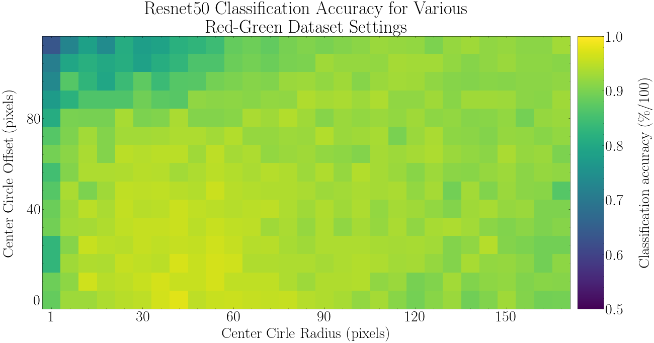
6. Discussion
92% mean accuracy compared to 81% for the orange-brown dataset. I think an implication of these results is that if one is using this pretrained ResNet model via transfer-learning and the final layer is retrained only, then the model may have a harder time classifying if the decision depends on orange-brown distinctions rather than green-red distinctions.