
Experiment 2. Summary.
Overview of progress in experiment 2.Motivation
Experiment 2 tries to see if there is anything interesting to say about how classification models behave in various illumination.
The nature of CNN receptive fields is what hints at their being something interesting to find. Look at the following crop of an image and consider what colors you see:
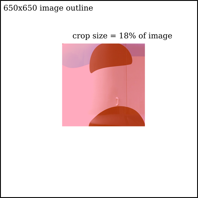
And now view the full image.
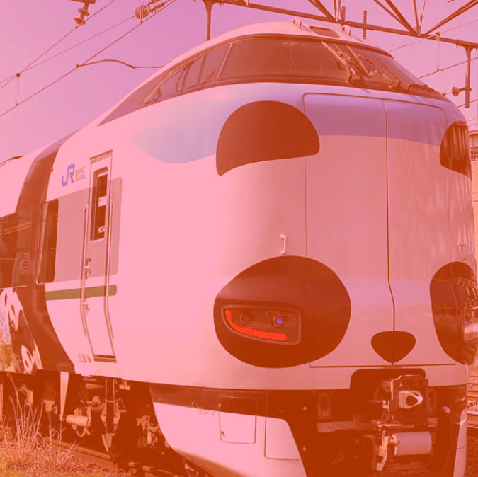
For me, what appears black-ish in the full image appears more like red in the cropped image. My brain uses the surrounding area of the image to estimate the illumination and then discount the illumination in order to give an interpretation of the reflectance properties of the black/red surface. The demo shows that quite a large area of the image contributes to the interpretation of small areas. Below is an outline showing the receptive field size of some of the layers of the ResNet50 model.

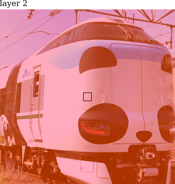

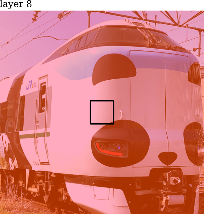
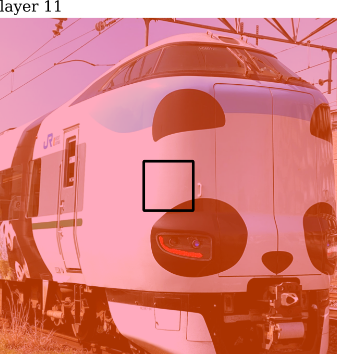
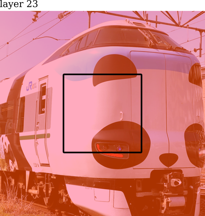
The receptive field size of the 23rd layer is a similar size to the cropped area. The 23rd layer is almost 1/2 way through the 50 layer network. This suggests that models such as ResNet50 might have not have a good model of the scene illumination, and thus surface reflectance properties, in their early layers.
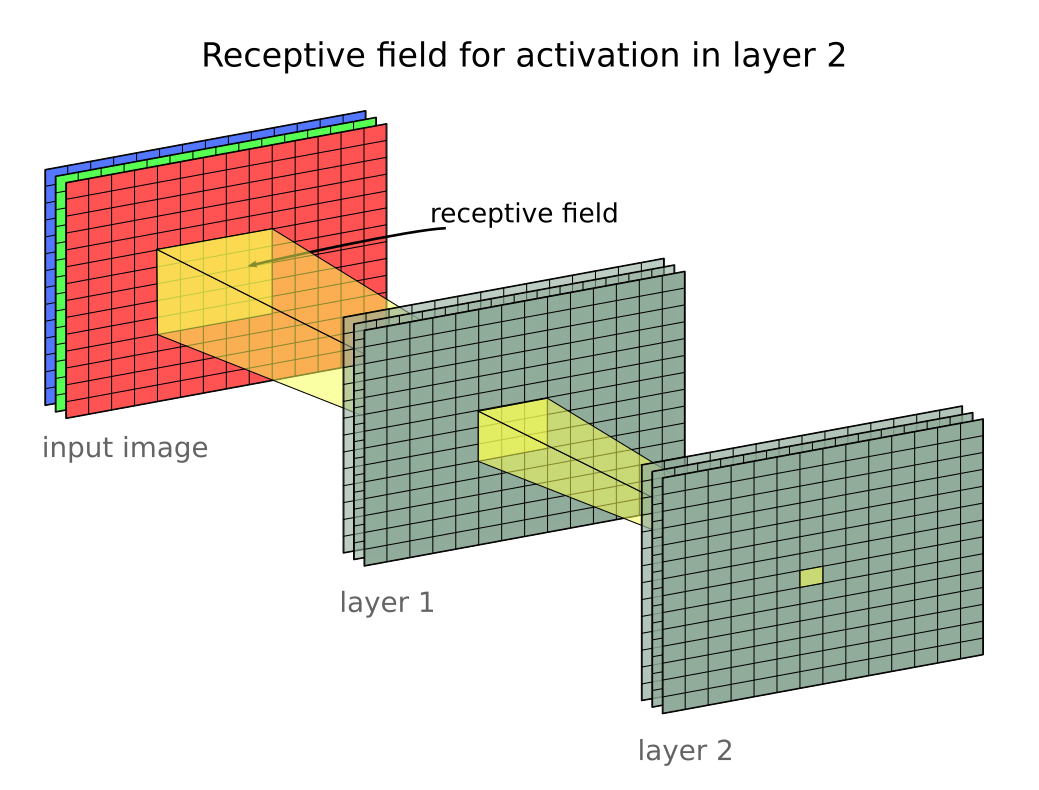
Receptive fields
The receptive field referred to in the previous paragraph is referring to the following property of CNNs:
Experiment 2.1.1 and 2.1.2
These two experiments investigated how illumination changes effect ResNet image classification.
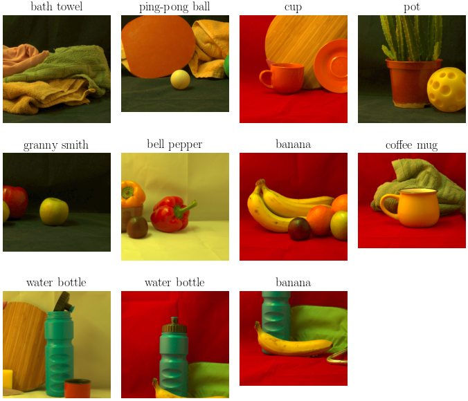
The data used is the following 11 scenes:
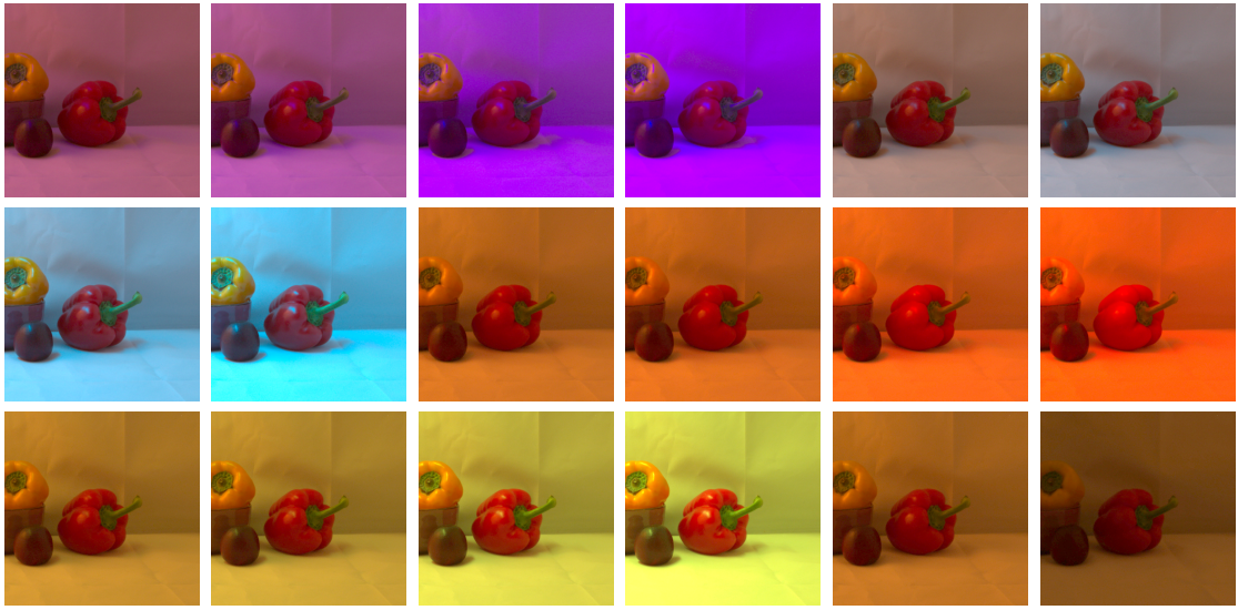
For each scene, there are 18 illuminations. Here are all 18 for the capsicum scene:
The interesting result to come from these experiments is the following effect of varying illumination:
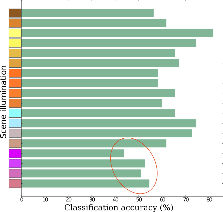
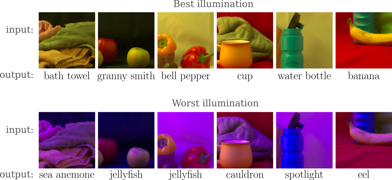
The y-axis labels are suggestive but not accurate representations of the illumination. The lighting with strong blue-LEDs produces relatively poor classification accuracy. Comparing the best and worst illumination, we have the following results for when the model is incorrect under the worst illumination and correct under the best illumination:
Experiment 3.2
Experiment 3.2 applies the grayworld algorithm to the images before sending them to the model. The algorithm is a very simple illumination discounting (white balancing) algorithm.
The results of this setup compared to the original experiment:
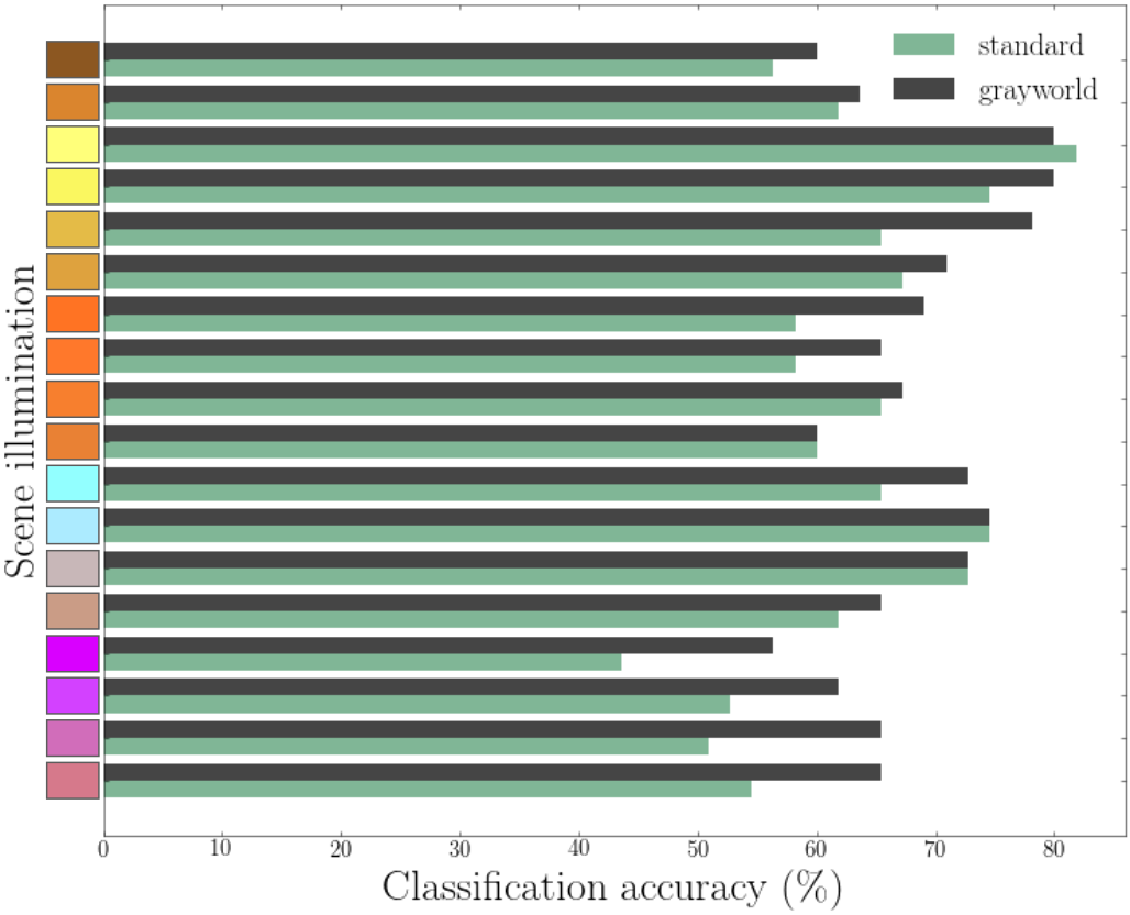 Quite an effect!
Experiment 3.3
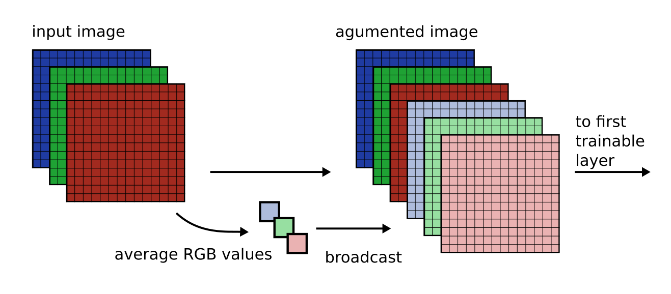
This experiment (not yet uploaded) is investing including the grayworld idea as a prior by adding 3 new channels to the first layer of the model. Each channel carries the average R, G and B color value of the input image. This alteration is hoped to give the model information about the whole image that might enable it to estimate illumination earlier in the network.
The idea is depicted as follows:
Preliminary results hint at some of the interesting developments:
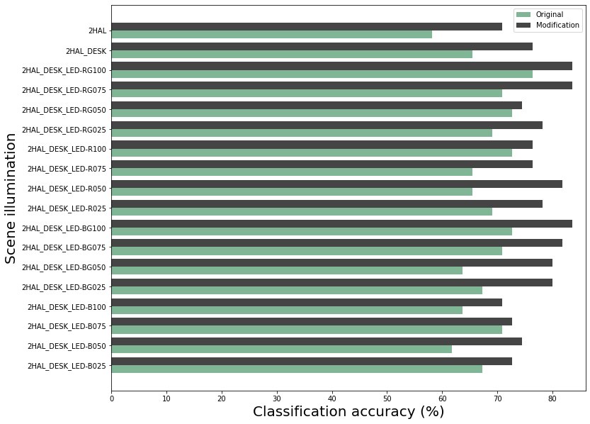
The “original” accuracies don’t look like the ones above, these two model were trained with different training procedures. So, the first observation is that training procedures have an impact on illumination invariance. The training proceedure that seemed to have a significant effect was the mixup augmentation.
Even though the newly trained ResNet50 model has improved illumination invariance without the grayworld modification, we still see an improvement when the modification is added.