
Cross-Entropy and KL divergence
Consider that we have an encoding scheme for sending codewords from a set \( C \) whose frequencies are given by the probability distribution \( q: C \to \mathbb{R} \). Assume that this scheme achieves the minimum average message length possible. The minimum possible average message length for any such encoding is equal to the entropy of the distribution, given by the equation:
Here, the syntax presents \( H \) as an operator taking in a distribution over \( C \).
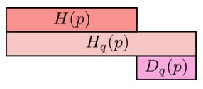
Now, imagine that the same codewords are sent, but the frequency distribution of the codewords is changed to \( p: C \to \mathbb{R} \); the codewords are no longer optimized to the distribution. The new average length is given by the cross-entropy of \( q \) relative to \( p \):
\( H_q(p) \) is also as an operator taking in a distribution over \( C \). Keeping this in mind helps remember the placement of \( q \) and \( p \) in the syntax \( H_q(p) \).
The length of a codeword is still the same (\( \log_2(\frac{1}{q(x)}) \)) , but the probability of the codeword being sent/received has changed to \( p(x) \). The cross-entropy is always larger than the entropy of the original distribution. If we were to then update our encoding to a better \( p \)-optimized encoding, our average message length would decrease from \( H_q(p) \) to \( H(p) \).
KL divergence (a pseudo-difference measure between distributions)
Cross-entropy gives us a way to express how different two probability distributions are; the more different the distributions \( p \) and \( q \) are, the more the cross-entropy of \( q \) with respect to \( p \) will be bigger than the entropy of \( p \).
And the same goes for the cross-entropy of \( p \) with respect to \( q \):
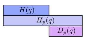
The differences, \( D_q(p) \) and \( D_p(q) \) are called Kullback-Leibler divergences (KL divergence). The KL divergence from \( q \) to \( p \), \( D_q(p) \) is defined as:
In words
The average message length reduction of using a \( q \)-optimized encoding when the transmission distribution is \( p \), then switching to a \( p \)-optimized encoding; this is the KL divergence from \( q \) to \( p \).
Distance-like
The KL divergence is like a distance between two distributions; however, the KL divergence is not symmetric: it is possible for \( D_p(q) \neq D_q(p) \), so it is not a true distance measure. Often in machine learning we want one distribution to be close to another. Minimizing the KL divergence is a natural way to minimize the distance between two distributions.
The formulation of KL-divergence
There are two ways of thinking about the change in message length: you have an encoding, then the transmission distribution changes, or the transmission distribution stays the same and you switch encodings. The first situation might suggest a measure of difference like:
The KL-divergence represents the second situation (changing encoding with fixed transmission distribution):
(average length of the q-optimized encoding under p) - (average length of the p-optimized encoding under p)
The KL divergence makes more sense when viewed as a calculation, as the summations share the same factor:
Compare this to the calculation required for the first formulation:
This can't be simplified in the same way as the KL divergence can.